Getting Started

This section is going to show you how to use the NiaARM framework.

Installation

You can install NiaARM package using the following command:

pip install niaarm

Usage

Loading Data

In NiaARM, data loading is done via the Dataset class. There are two options for loading data:

Option 1: Directly from file

from niaarm import Dataset

dataset = Dataset('Abalone.csv')
print(dataset)

Option 2: From a pandas DataFrame (recommended)

This option is recommended, as it allows you to preprocess the data before mining.

import pandas as pd
from niaarm import Dataset


df = pd.read_csv('Abalone.csv')
# Preprocess the dataframe...
dataset = Dataset(df)
print(dataset)

Output:

DATASET INFO:
Number of transactions: 4177
Number of features: 9

FEATURE INFO:

                    Sex Length Diameter Height Whole weight Shucked weight Viscera weight Shell weight Rings
dtype       categorical  float    float  float        float          float          float        float   int
min_val             N/A  0.075    0.055    0.0        0.002          0.001         0.0005       0.0015     1
max_val             N/A  0.815     0.65   1.13       2.8255          1.488           0.76        1.005    29
categories    [M, F, I]    N/A      N/A    N/A          N/A            N/A            N/A          N/A   N/A

Preprocessing

The preprocessing module provides functions for preprocessing transaction data. The only preprocessing method currently implemented is the squash() method, presented in this paper.

from niaarm.dataset import Dataset
from niaarm.preprocessing import squash


dataset = Dataset('datasets/Abalone.csv')
squashed = squash(dataset, threshold=0.9, similarity='euclidean')
print(squashed)

Output:

DATASET INFO:
Number of transactions: 626
Number of features: 9

FEATURE INFO:

                  Sex Length Diameter Height Whole weight Shucked weight Viscera weight Shell weight Rings
dtype        category  float    float  float        float          float          float        float   int
min_val           N/A  0.075    0.055    0.0        0.002          0.001         0.0005       0.0015     1
max_val           N/A  0.815     0.65   1.13       2.8255          1.488           0.76        1.005    29
categories  [F, I, M]    N/A      N/A    N/A          N/A            N/A            N/A          N/A   N/A

Mining Association Rules

Once the data has been loaded, we can run our mining algorithm.

The key component here is our NiaARM class, which inherits from NiaPy’s Problem class. It implements numerical association rule mining as a real valued, single objective, unconstrained maximization problem (more details on this approach can be found here and here). To summarize, for each solution vector a Rule is built, and it’s fitness is computed as a weighted sum of selected interestingness measures (metrics). The rule is then appended to a list of rules, which can be accessed through the NiaARM class.

The NiaARM class takes the dataset’s dimension (calculated dimension of the optimization problem), features, and transactions (all attributes of the Dataset class) and the metrics selected for the fitness function. The metrics can either be passed in as a sequence of strings, in which case the weights of the metrics will be set to 1, or you can pass in a dict containing pairs of {'metric_name': weight}. You can also enable logging of fitness improvements by setting the logging parameter to True.

Bellow is a simple example of mining association rules on the Abalone dataset that we loaded above. For this example we picked Differential Evolution, specifically DE/rand/1/bin, which we’ll be running for 50 iterations. All available algorithms can be found in the NiaPy documentation. We’ve selected the metrics: ‘support’, ‘confidence’, ‘inclusion’ and ‘amplitude’ for the fitness function. We then sort the rules by fitness in descending order and export them to csv.

from niaarm import NiaARM
from niapy.task import OptimizationType, Task
from niapy.algorithms.basic import DifferentialEvolution


# DE/rand/1/bin
algorithm = DifferentialEvolution(population_size=50,
                                  differential_weight=0.8,
                                  crossover_probability=0.9)

metrics = ('support', 'confidence', 'inclusion', 'amplitude')

problem = NiaARM(dataset.dimension, dataset.features, dataset.transactions, metrics, logging=True)
task = Task(problem, max_iters=50, optimization_type=OptimizationType.MAXIMIZATION)

algorithm.run(task)

problem.rules.sort(by='fitness', reverse=True)
problem.rules.to_csv('output.csv')

The mined rules are stored in problem.rules, a RuleList. A RuleList is a thin wrapper around a normal python list, with the added functionalities of sorting by metric, exporting rules to csv, and properties for getting statistical data about the rules. Printing a RuleList prints a statistical report of the rules in it.

Output:

Fitness: 0.4421065111459649, Support: 0.00023940627244433804, Confidence: 1.0, Inclusion: 0.3333333333333333, Amplitude: 0.43485330497808217
Fitness: 0.5363319939110781, Support: 0.006942781900885803, Confidence: 0.9354838709677419, Inclusion: 0.5555555555555556, Amplitude: 0.6473457672201293
Fitness: 0.5395969006117709, Support: 0.1812305482403639, Confidence: 0.9895424836601308, Inclusion: 0.4444444444444444, Amplitude: 0.5431701261021447
Fitness: 0.5560783231641568, Support: 0.0023940627244433805, Confidence: 1.0, Inclusion: 0.6666666666666666, Amplitude: 0.5552525632655172
Fitness: 0.5711107256845077, Support: 0.5997127124730668, Confidence: 1.0, Inclusion: 0.3333333333333333, Amplitude: 0.3513968569316307
Fitness: 0.5970815767218225, Support: 0.8099114196791956, Confidence: 0.9955856386109476, Inclusion: 0.3333333333333333, Amplitude: 0.2494959152638132
Fitness: 0.6479501714015481, Support: 0.7455111323916687, Confidence: 0.9860671310956302, Inclusion: 0.3333333333333333, Amplitude: 0.5268890887855602
Fitness: 0.6497709183879634, Support: 0.9820445295666747, Confidence: 1.0, Inclusion: 0.4444444444444444, Amplitude: 0.17259469954073503
Fitness: 0.6522418829904134, Support: 0.9176442422791478, Confidence: 0.9422320550639135, Inclusion: 0.4444444444444444, Amplitude: 0.304646790174148
Fitness: 0.6600433108204055, Support: 0.9762987790280105, Confidence: 1.0, Inclusion: 0.5555555555555556, Amplitude: 0.1083189086980556
Fitness: 0.6625114159138297, Support: 0.9209959300933684, Confidence: 1.0, Inclusion: 0.3333333333333333, Amplitude: 0.39571640022861654
Fitness: 0.6748446186051374, Support: 0.9916207804644481, Confidence: 0.9916207804644481, Inclusion: 0.4444444444444444, Amplitude: 0.27169246904720923
Fitness: 0.6868285539707781, Support: 0.949006463969356, Confidence: 0.9927372902579514, Inclusion: 0.5555555555555556, Amplitude: 0.25001490610024923
Rules exported to output.csv

Mining Association Rules (Simplified)

In addition to the above interface, we provide a much simpler one in the form of a simple function: get_rules. The function accepts a dataset object, an algorithm, sequence or dict of metrics, a stopping condition (either max_evals or max_iters) and a logging flag. The algorithm can either be a NiaPy Algorithm instance, or a string, in which case it’s parameters can be passed in to the function as additional keyword arguments.

The get_rules function returns a named tuple of (rules, run_time), where rules is a RuleList and run_time is the run time of the algorithm in seconds.

The same example as above, using get_rules:

from niaarm import get_rules
from niapy.algorithms.basic import DifferentialEvolution


# DE/rand/1/bin
algorithm = DifferentialEvolution(population_size=50,
                                  differential_weight=0.8,
                                  crossover_probability=0.9)

metrics = ('support', 'confidence', 'inclusion', 'amplitude')
rules, run_time = get_rules(dataset, algorithm, metrics, max_iters=50)
print(rules)
print(f'Run Time: {run_time:.4f} seconds')
rules.to_csv('output.csv')

Output:

STATS:
Total rules: 1153
Average fitness: 0.47320577312454054
Average support: 0.3983325861836626
Average confidence: 0.7050696319555724
Average lift: 1.8269022321777044
Average coverage: 0.5791478590164908
Average consequent support: 0.6708142990119975
Average conviction: 80294763647830.92
Average amplitude: 0.33832710930158877
Average inclusion: 0.45109376505733834
Average interestingness: 0.4107718184209992
Average comprehensibility: 0.6225319999993354
Average netconf: 0.08165217509315073
Average Yule's Q: 0.2631267094311884
Average length of antecedent: 2.248048568950564
Average length of consequent: 1.8117953165654814
Run Time: 6.9498 seconds
Rules exported to output.csv

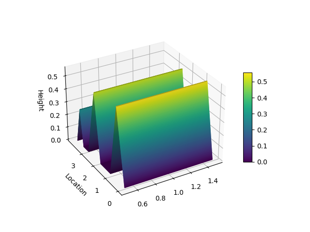
Visualization

The visualize module provides functions for plotting association rules. The only visualization method currently implemented is the hill_slopes() method, presented in this paper.

from matplotlib import pyplot as plt
from niaarm import Dataset, RuleList, get_rules
from niaarm.visualize import hill_slopes

dataset = Dataset('datasets/Abalone.csv')
metrics = ('support', 'confidence')
rules, _ = get_rules(dataset, 'DifferentialEvolution', metrics, max_evals=1000, seed=1234)
some_rule = rules[150]
hill_slopes(some_rule, dataset.transactions)
plt.show()

Output:

Text Mining (Experimental)

An experimental implementation of association rule text mining using nature-inspired algorithms is also provided. The niaarm.text module contains the Corpus and Document classes for loading and preprocessing corpora, a TextRule class, representing a text rule, and the NiaARTM class, implementing association rule text mining as a continuous optimization problem. The get_text_rules() function, equivalent to get_rules(), but for text mining, was also added to the niaarm.mine module.

import pandas as pd
from niaarm.text import Corpus
from niaarm.mine import get_text_rules
from niapy.algorithms.basic import ParticleSwarmOptimization

df = pd.read_json('datasets/text/artm_test_dataset.json', orient='records')
documents = df['text'].tolist()
corpus = Corpus.from_list(documents)

algorithm = ParticleSwarmOptimization(population_size=200, seed=123)
metrics = ('support', 'confidence', 'aws')
rules, time = get_text_rules(corpus, max_terms=5, algorithm=algorithm, metrics=metrics, max_evals=10000, logging=True)

if len(rules):
    print(rules)
    print(f'Run time: {time:.2f}s')
    rules.to_csv('output.csv')
else:
    print('No rules generated')
    print(f'Run time: {time:.2f}s')

Note: You may need to download stopwords and the punkt_tab tokenizer from nltk by running import nltk; nltk.download(‘stopwords’); nltk.download(‘punkt_tab’).

Output:

Fitness: 0.53345778328699, Support: 0.1111111111111111, Confidence: 1.0, Aws: 0.48926223874985886
Fitness: 0.7155830770302328, Support: 0.1111111111111111, Confidence: 1.0, Aws: 1.0356381199795872
Fitness: 0.7279963436805833, Support: 0.1111111111111111, Confidence: 1.0, Aws: 1.072877919930639
Fitness: 0.7875917299029188, Support: 0.1111111111111111, Confidence: 1.0, Aws: 1.251664078597645
Fitness: 0.8071206688346807, Support: 0.1111111111111111, Confidence: 1.0, Aws: 1.310250895392931
STATS:
Total rules: 52
Average fitness: 0.5179965084882088
Average support: 0.11538461538461527
Average confidence: 0.7115384615384616
Average lift: 5.524038461538462
Average coverage: 0.17948717948717943
Average consequent support: 0.1517094017094015
Average conviction: 1568561408678185.8
Average amplitude: nan
Average inclusion: 0.007735042735042727
Average interestingness: 0.6170069642291859
Average comprehensibility: 0.6763685578758655
Average netconf: 0.6675824175824177
Average Yule's Q: 0.9670329670329672
Average antecedent length: 1.6346153846153846
Average consequent length: 1.8461538461538463

Run time: 13.37s
Rules exported to output.csv

Interestingness measures

The framework currently implements the following interestingness measures (metrics):

• Support

• Confidence

• Lift [1]

• Coverage

• RHS Support

• Conviction [1]

• Inclusion

• Amplitude

• Interestingness

• Comprehensibility

• Netconf [1]

• Yule’s Q [1]

• Zhang’s Metric [1]

More information about these interestingness measures can be found in the API reference of the Rule class.

Footnotes

[1] (1,2,3,4,5)

Not available as fitness metrics.

Examples

You can find the full code and usage examples here.